引言
TT-Buda 是一个高层次软件栈,它可以兼容各种人工智能框架,并采用自顶向下的方式,生成可执行文件以便在 Tenstorrent 硬件上运行人工智能模型。
整体架构
整体架构分析
AI模型在tt-buda架构下的编译执行过程如下图所示:
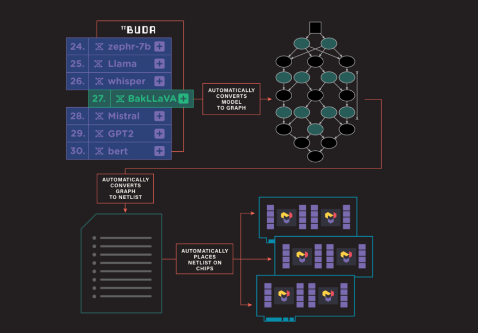
图 1:tt-buda 编译执行过程(来源:Tenstorrent)
流程分三个部分:
-
根据AI模型生成计算图
-
计算图转换成Netlist(网表)
-
Netlist映射到具体设备
详细过程展开如下图所示:
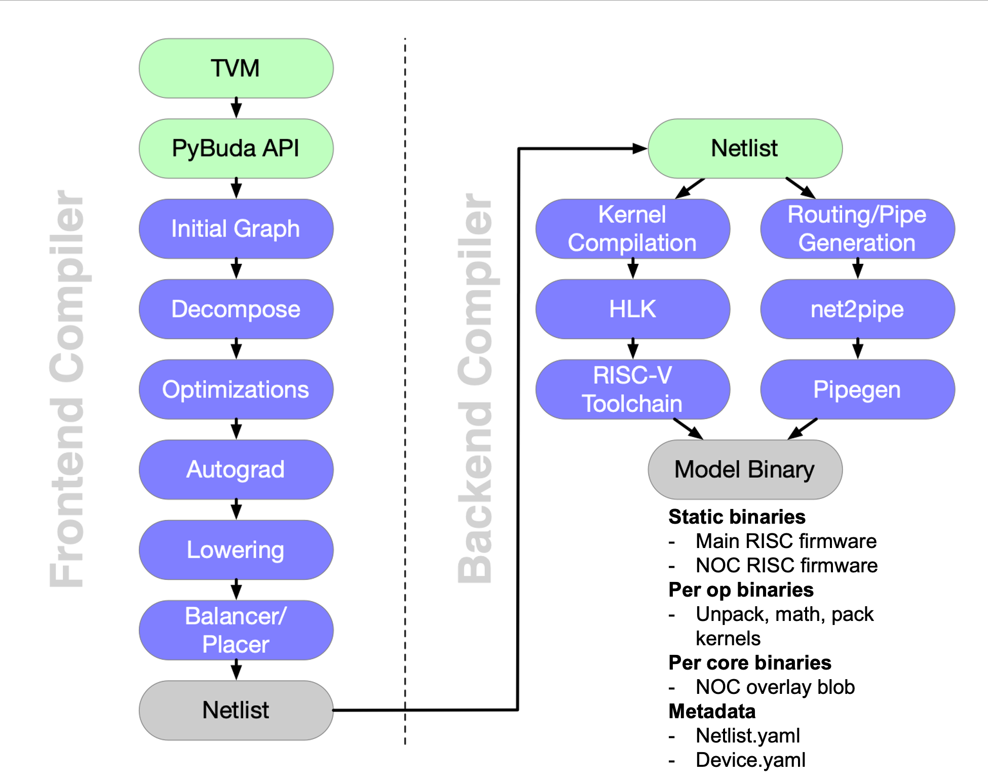
图 2:tt-buda software stack overview(来源:Tenstorrent)
与其他AI编译器一样,tt-buda也分为frontend和backend两个部分。区别在于,tt-buda使用Netlist作为中间表示形式,连接frontend和backend。
Frontend
AI模型(使用其他框架开发的)通过TVM转换成PyBuda API,然后生成计算图,经过优化、自动微分、Lowering、Balancer/Placer,最后生成Netlist。
除了上图所示的第三方AI模型外,还可以使用pybuda api开发PyBuda模型。PyBuda模型可以直接转换成计算图,不需要经过TVM。
Backend
Backend功能完全由budabackend实现,分为两个部分:
-
生成可执行文件:将Netlist中描述的算子(op)翻译成HLK(high level kernel,高层次算子),然后调用自定义的RISC-V编译器(gcc),将算子编译成可执行文件(包含RISC-V标准指令和自定义指令)。
-
生成路由文件:将Netlist中描述的数据传输信息,通过工具net2pipe和pipegen,翻译成 NOC overlay blob(一种硬件配置文件,供硬件传输单元使用)。
衔接前后端的文件 – Netlist
Netlist 是 tt-buda 软件栈的中间表示,格式为 YAML 文件。它描述了 BUDA 后端的工作负载,包含了几个组成部分:设备、队列、图、操作(op)、程序等等(详细分析见下期教程)。
使用和开发实践
下面分析两个简单的例子,介绍 runtime API 的使用方法。第一个例子兼容现有的模型,第二个例子使用 pybuda API 开发简单的模型。
示例1 – Bert
# example1: sample way to run model
import pybuda
import torch
from transformers import BertModel, BertConfig

# Download the model from huggingface
model = BertModel.from_pretrained("bert-base-uncased") # 1

# Wrap the pytorch model in a PyBuda module wrapper
module = pybuda.PyTorchModule("bert_encoder", model.encoder) # 2

# Create a tenstorrent device
tt0 = pybuda.TTDevice(
    "tt0",
    module=module,
    arch=pybuda.BackendDevice.Wormhole_B0,
    devtype=pybuda.BackendType.Silicon,
) # 3

# Create an input tensor
seq_len = 128
input = torch.randn(1, seq_len, model.config.hidden_size)

# Compile and run inference
output_queue = pybuda.run_inference(inputs=[input]) # 4
print(output_queue.get())
分析上述源码,预编译模型的运行有以下几步:
-
从 huggingface 下载预编译模型
-
使用 PyBuda module 包装模型
-
创建 tenstorrent device
-
在设备上运行模型
pybuda.run_inference 是一键推理接口,会自动识别已有的设备。设备类型有 CPUDevice 和 TTDevice(tenstorrent设备,Grayskull、Wormhole),如果存在 TTDevice 不支持的算子,那么需要将算子映射到 CPUDevice(可以通过编译参数控制自动执行,而不需要手动创建 CPUDevice)。pybuda.PyTorchModule 是 Pytorch 模型的 Wrapper,使用外部框架模型前,需要使用包装器封装一下。
以下是支持的第三方模型框架:
| Framework | PyBuda Wrapper Class | Support |
| Pybuda | pybuda.PyBudaModule |
Native Support |
| Pytorch | pybuda.PyTorchModule |
Supported |
| Tensorflow | pybuda.TFModule |
Supported |
| Jax | pybuda.JaxModule |
Supported via jax2tf |
| Tensorflow Lite | pybuda.TFLiteModule |
Preliminary Support |
| Onnx | pybuda.OnnxModule |
Preliminary Support |
| Tensorflow GraphDef | pybuda.TFGraphDefModule |
Preliminary Support |
可以看出,tt-buda 对第三方框架的兼容性很好,Pytorch和Tensorflow完全支持,Onnx和Tensorflow Lite部分支持。
Bert模型运行结果
为了方便比较Grayskull和GPU (RTX 3090)运行模型的结果,使用tenstorrent开源项目benchmarking进行比较。
// 在tenstorrent硬件上运行bert模型
$ python benchmark.py -d tt -m bert -c large --task text_classification -mb 64 --loop_count 4 --save_output
// 在nvidia GPU上运行bert模型
$ python3 benchmark.py -d cuda -m bert -c large --task text_classification -mb 64 --loop_count 4 --save_output
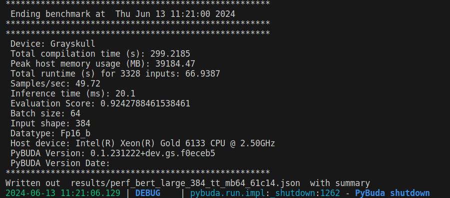
图 3:bert在Grayskull上运行日志
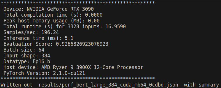
图 4:bert在nvidia RTX3090上运行日志
对比bert模型在Grayskull和nvidia RTX3090上运行的结果,会发现Grayskull比3090慢4倍,原因在于单张Grayskull卡资源有限,bert模型太大,导致模型无法在单张卡上高效的展开。查看bert编译的netlist可知,模型被划分成了74个epoch,每个epoch仅仅使用了少量的Tensix(远少于120个),每当epoch切换的时候,需要将结果写回到DRAM,新的数据、可执行程序、路由文件从DRAM拷贝到L1,导致了效率差,查看运行日志可以佐证这一点,大量的时间花费在了queue的写入和写出。
示例2 – PyBuda matmul
import pybuda
import pybuda.op
import torch
from pybuda import PyBudaModule, TTDevice

# Create a simple matmul transformation module
class BudaMatmul(PyBudaModule):
  def __init__(self, name):
      super().__init__(name)
      self.weights = pybuda.Parameter(1, 1, 32, 32, requires_grad=False)
  def forward(self, act):
      return pybuda.op.Matmul(self, "matmul", act, self.weights)

if __name__ == '__main__':
    tt0 = TTDevice("grayskull0")   # Create a Tensorrent device
    lin0 = BudaMatmul("matmul0")   # Instantiate the above model
    tt0.place_module(lin0)         # Place the model on TT device

    act = torch.rand(1, 1, 32, 32) # Feed some random data to the device
    tt0.push_to_inputs(act)

    results = pybuda.run_inference(num_inputs=1, sequential=True)  # Run inference and collect the results
示例2自定义了一个Pybuda模型,对比示例1,示例2手动调用了 place_module(将module放置到指定设备)和 push_to_inputs(将数据push到输入队列)。而且,示例2使用自定义 class BudaMatmul 继承自 PyBudaModule,参数在构造函数中定义,操作在 forward 方法中定义。pybuda.op.Matmul 是一个python层的算子API,是对HLK(high level kernel)层的一种封装。
现有模型的使用
当软硬件环境就绪,可以直接运行tt-buda已支持的模型,这些模型放置在third_party/model_demos 目录。
运行 pytorch_mobilenet_v1:
$ python third_party/buda-model-demos/model_demos/cv_demos/mobilenet_v1/pytorch_mobilenet_v1_basic.py
运行完毕后,会在当前目录生成一些文件
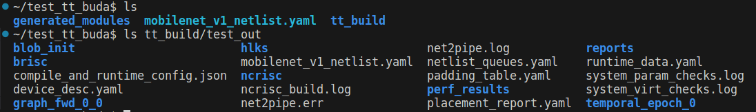
图 5:tt-buda 运行模型后生成文件
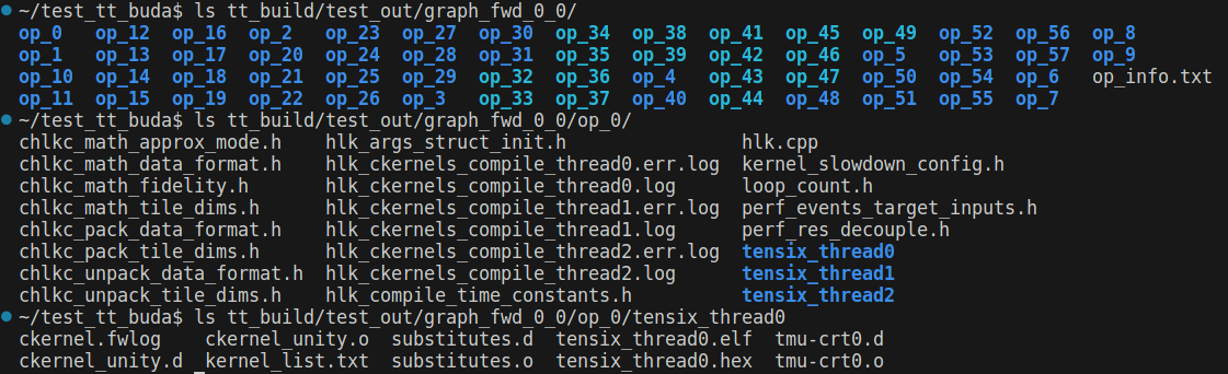
图 6:tt-buda 运行模型后生成文件,graph和op
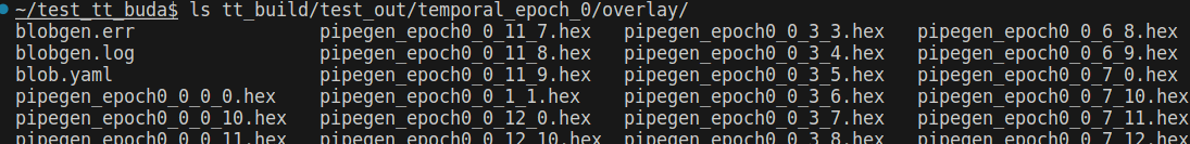
图 7:tt-buda 运行模型后生成文件,overlay文件
其中,除去一些日志文件和中间文件以外,较为重要的文件有:
-
mobilenet_v1_netlist.yaml – 网表文件,保存了op的映射关系和路由信息。
-
hlks – high level kernel 保存每个op对应的源码。
-
graph_fwd_0_0 – 如图6所示,保存了图和op的信息。每个op包含三个thread,对应了 unpack、math、pack 三个不同的功能,thread有自己的可执行文件 tensix_thread*.elf。
-
temporal_epoch_0/overlay – 如图7所示,overlay配置文件,由pipegen工具生成,每个Tensix都有自己的一份,包含路由信息。
每个Tensix有5个baby riscv core,每个core有自己的分工(分工详细见Tenstorrent数据流芯片Grayskull 和 Wormhole解析Tensix部分),所以也都有自己的可执行文件。BRISC和NCRISC的可执行文件是固定的(保存在图3的brisc/ncrisc目录),具体数据路由信息保存在overlay配置文件中。
源码分析
源码目录结构
tt-buda的源码目录结构如下:
$ tree -d -L 2
├── ci
│   └── gitlab-test-lists
├── docs
│   ├── CI
│   └── public
├── pybuda
│   ├── csrc
│   ├── pybuda
│   └── test
├── python_env
├── scripts
├── third_party
│   ├── budabackend
│   ├── buda-model-demos
│   ├── fmt
│   ├── json
│   ├── pybind11
│   └── tvm
└── utils
    └── ordered_associative_containers
比较重要的部分有:
-
pybuda/csrc:包含 autograd、balancer、placer、passes 等,是实现 frontend 部分功能的核心代码
-
pybuda/pybuda:runtime,负责调用 tvm 和 budabackend 进行编译,以及模型的加载和执行
-
third_party/budabackend:编译器后端,负责将 Netlist 编译成设备上的可执行文件和路由文件
-
third_party/tvm:TVM编译器,用于兼容其他框架编写的模型,将其转换成 pybuda API
tvm 和 budabackend 以 submodule 的模式嵌入到 tt-buda 项目中,pybuda 集合了 runtime 和 frontend compiler 的功能,runtime 部分使用 python 进行开发,frontend 部分使用 c++ 开发。
PyBuda runtime
如上面的示例所示,pybuda runtime 提供了一套面向用户的 API,可以用于加载或开发模型。frontend、backend、tvm 通过 pybind 提供一套 python API,runtime 调用 python API 完成具体的功能。为了更好的理解 tt-buda 运行模型的过程,不妨追踪一下 pybuda.run_inference 函数调用。
run_inference
 └── _run_inference
        └── _run_devices_inference
             └── _initialize_pipeline
                 └── _compile_devices
                     └── compile
                         └── compile_for
                             └── pybuda_compile_from_context
展开 pybuda_compile_from_context 函数,部分代码如下:
    # Map stages to functions which execute them.
    stage_to_func = {
        CompileDepth.INIT_COMPILE: init_compile,
        CompileDepth.GENERATE_INITIAL_GRAPH: generate_initial_graph,
        CompileDepth.POST_INITIAL_GRAPH_PASS: run_post_initial_graph_pass,
        CompileDepth.CONSTEVAL_GRAPH: run_consteval_pass,
        CompileDepth.POST_PATTERN_MATCHER: run_post_pattern_matcher,
        CompileDepth.OPTIMIZED_GRAPH: run_optimization_pass,
        CompileDepth.AUTOGRAD: run_autograd_pass,
        CompileDepth.POST_AUTOGRAD_PASS: run_post_autograd_pass,
        CompileDepth.PRE_LOWERING_PASS: run_pre_lowering_pass,
        CompileDepth.BUDA_GRAPH_PRE_PLACER: run_pre_placer_pass,
        CompileDepth.BALANCER_PASS: run_balancer_and_placer,
        CompileDepth.PRE_NETLIST_PASS: run_pre_netlist_pass,
        CompileDepth.GENERATE_NETLIST: generate_netlist,
        CompileDepth.BACKEND_GOLDEN_VERIFY: run_backend_golden_verify,
    }
可以看出,frontend 编译过程是分阶段进行的(对应图2),每个阶段对应一个回调函数。
分析回调函数 run_balancer_and_placer 如下所示,最终会从python接口调用到c++实现的函数。
run_balancer_and_placer
    └── run_placer_buda_passes // 在c++中实现,使用pybind展现python接口
        └── balancer::run_balancer_and_placer // pybuda/csrc/placer/placer.cpp
balancer/placer 的作用是将初始化的计算图进行负载平衡,映射到硬件上的计算单元上。
run_balancer_and_placer
Transformer 映射到 tensix cores 示意图如下:
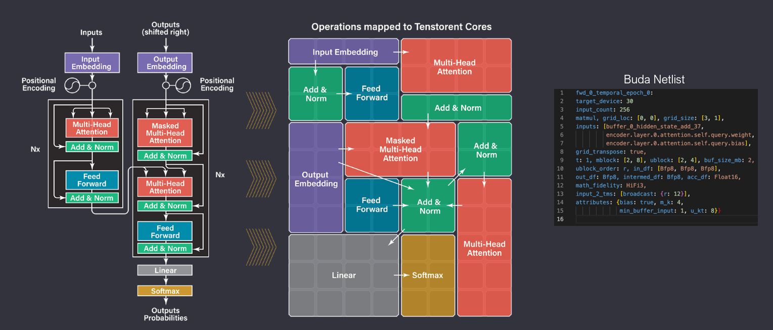
图 8:transformer 映射到 tensix cores
模型中计算量大的层会被映射到更多的Tensix,这种映射关系由balancer/placer决定。
run_balancer_and_placer 的关键逻辑如下:
LegalOpModels valid_op_models = legalizer::get_legal_op_models(graph, config, cache_collection);
legalizer::GraphSolver graph_solver = get_graph_solver(config, cache_collection, graph, valid_op_models);
BalancerPolicySolution balancer_policy_solution = run_policy(graph, config, graph_solver);
OpModel 用于保存 op 的相关信息,如 id、dataformat、grid_shape(grid代表的是Tensix的坐标,grid_shape用于描述使用哪几个Tensix用于执行当前op)、buffers(输入输出数据地址)等等。get_legal_op_models 会将所有合法的 op 和 OpModel 键值对保存在 valid_op_models,然后调用 get_graph_solver 对图进行分割,最后根据不同的平衡策略(Balancer policy)选择映射关系。
Balancer policy 有以下几种:
-
MaximizeTMinimizeGrid
-
MinimizeGrid
-
Random
-
NLP
-
CNN
-
Ribbon
除了最小化和随机策略以外,还有针对模型的特化策略,每种策略对应一个回调函数,以下是最小化策略实现:
BalancerPolicySolution run_policy_minimize_grid(Graph const* graph, BalancerConfig const&, legalizer::GraphSolver& graph_solver)
{
    for (Node* node : tt::graphlib::topological_sort(*graph)) {
        auto legal_op_models = graph_solver.at(node);
        std::vector<OpModel> op_models(legal_op_models.begin(), legal_op_models.end());
        std::sort(
            op_models.begin(),
            op_models.end(),
            [](OpModel const& a, OpModel const& b) -> bool
            {
                int perimeter_a = a.grid_shape.r + a.grid_shape.c;
                int perimeter_b = b.grid_shape.r + b.grid_shape.c;
                if (perimeter_a == perimeter_b)
                    return a.grid_shape.r < b.grid_shape.r;
                return perimeter_a < perimeter_b;
            });
        graph_solver.set(node, op_models.front());
  }
    return BalancerPolicySolution(graph_solver.finish());
}
该策略选取了使用最少 Tensix 的映射方式。
其他特性
Multiple devices
TTDevice 可表示任意数量的设备集合,它允许使用不同的初始化方式,来选择不同的硬件。
tt0 = TTDevice("tt0") # num_chips=0
tt0 = TTDevice("tt0", num_chips=3)
tt0 = TTDevice("tt0", chip_ids[0, 2, 3])
指定 chip_ids 可以选择指定 id 的设备,指定 num_chips 选择指定数量的可用设备,当 num_chips 和 chip_ids 都不指定时,默认检测并使用所有的可用设备(不同类型的设备,如grayskull和wormhole不能混合使用)。
TensTorrent Device Image (TTI)
Tenstorrent 映像 (TTI) 是一种独立存档文件,用于存储模型编译信息。它包含设备配置、编译器配置、编译后模型工件、后端构建文件和模型参数张量。
TTI 具有以下优点:
-
离线目标编译:无需目标设备即可编译模型。
-
快速启动:直接执行模型,无需编译。
-
易于共享:可在不同环境之间共享 TTI 存档。
-
灵活的序列化:支持自定义模型参数序列化格式。
如下所示,可以调用函数 compile_to_image 将模型编译成 image 文件,保存在本地。
tt0 = pybuda.TTDevice(
  name="tt0",
  arch=BackendDevice.Wormhole_B0,
  devtype=BackendType.Silicon
)
tt0.place_module(...)
device_img: TTDeviceImage = tt0.compile_to_image(
    img_path="device_images/tt0.tti",
    training=training,
    sample_inputs=(...),
)
image 文件被保存在 device_images/tt0.tti,里面的内容包括:
/unzipped_tti_directory
├── device.json # Device state and compiled model metadata
├── <module-name>.yaml # netlist yaml
├── compile_and_runtime_config.json # compiler and runtime configurations
├── backend_build_binaries # backend build binaries
│   ├── device_desc.yaml
│   ├── cluster_desc.yaml
│   ├── brisc
│   ├── erisc
│   ├── nrisc
│   ├── hlks
│   ├── epoch_programs
├── tensors # directory containing serialized tensors
├── module_files # Python file containing the PybudaModule of the model
除了编译生成的网表、可执行文件、路由信息等以外,tti 还包含模型文件 module_file 和输入数据 tensors。
加载和使用 tti 文件的方法如下:
img = TTDeviceImage.load_from_disk(img_path="device_images/tt0.tti")
device = TTDevice.load_image(img=img)

inputs = [torch.rand(shape) for shape in img.get_input_shapes()] # create tensors using shape info from img
device.push_to_inputs(inputs) # push newly created input activation tensors to device
output_q = pybuda.run_inference()
Automatic Mixed Precision(自动混合精度) & Math Fidelity(数学保真度)
混合精度计算通过结合高精度和低精度浮点数,能够在保持模型性能和精度的同时,大幅提高计算效率。pybuda 允许用户使用配置设置 AMP 等级,默认等级是0(禁用),不同的 AMP 对应不同的数学保真度策略,数学保真度越高,结果越准确,但所需的计算周期也越多。
总结
本文概述了 TT-Buda 的整体架构以及如何使用 TT-Buda 进行 AI 模型开发和加载。后续教程将详细介绍 Netlist 格式、算子实现(高级内核、低级内核)和路由文件等内容。
参考链接
【2】tt-buda官方文档